How it looks like

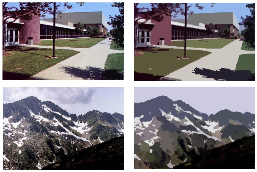
Our goal is to break up the image into similar regions without training data.

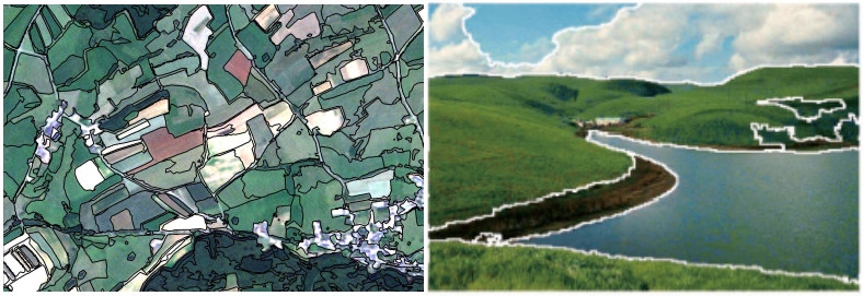
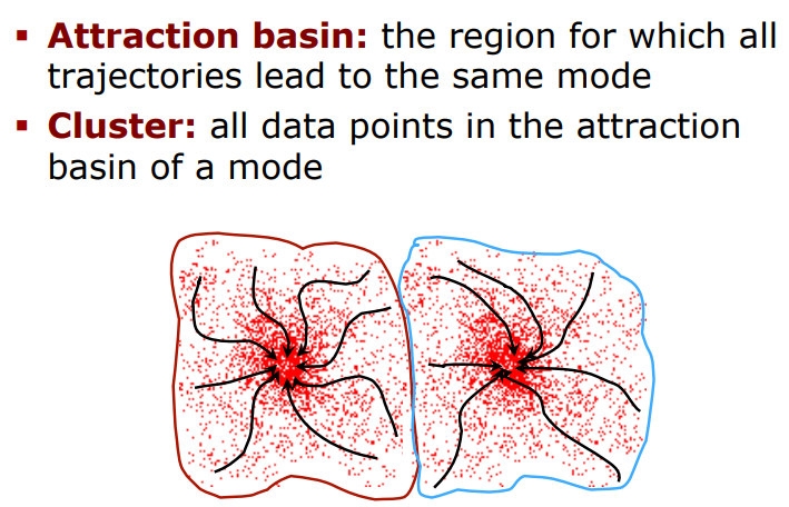
Try to find modes with a non-parametric density:

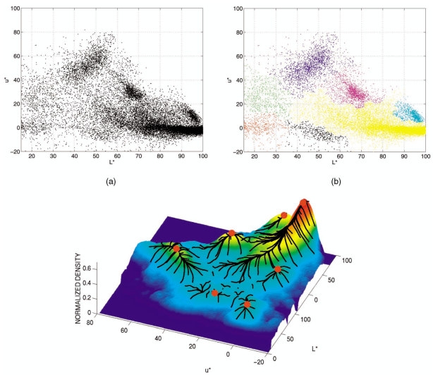
Mean Shift: A Robust Approach toward Feature Space Analysis, D.Comniciu and P.Meer

Idea: Estimating the PDF and Finding the Maxima

• Non-parametric approach to density estimation ("how many data points are in a certain region?")
• Find the local modes of this density
• All points that "belong" or "lead" to the same mode form a cluster

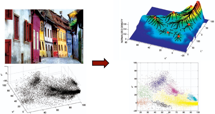
Mean Shift: A Robust Approach toward Feature Space Analysis, D.Comniciu and P.Meer

But how to estimate a PDF in non-parametric way?

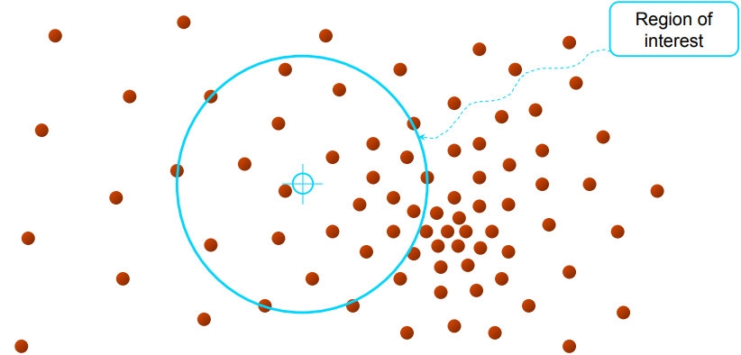
Using KDE, of course! The gold standard is Gaussian kernel.

И так происходит приближение к центру к центру, пока центр региона интереса не совпадает с центром массы:

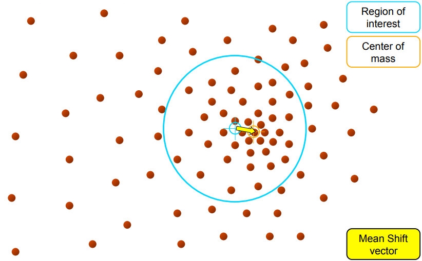
Упрощенно:

1. Compute mean shift vector
2. Move the kernel window

Segmentation

• Compute features for each pixel (color, gradients, texture, etc.)
• Set kernel size for features Kf and position Ks
• Initialize windows at individual pixel locations
• Perform mean shift for each window until convergence
• Merge windows that are within width of Kf and Ks

Mean Shift: A Robust Approach toward Feature Space Analysis, D.Comniciu and P.Meer

Understanding the Mean Shift Algorithm in Depth

Mean shift is a versatile technique for clustering-based segmentation of image data.

The mean shift algorithm is one of those hidden gems in the machine learning toolkit, especially loved for its simplicity and versatility in clustering and feature space analysis. In this blog post, we're going to break down the algorithm, dive deep into the math, look at Python implementations, and highlight its use cases. Expect a detailed discussion filled with LaTeX formulas for a math-centric view!

What is Mean Shift?

At its core, the mean shift algorithm is a non-parametric clustering method. It's called "mode-seeking" because its goal is to find the mode (or peak) of a density function, without needing to know how many clusters there are beforehand.

Unlike more traditional clustering methods like k-means, where we have to predefine the number of clusters ($k$), mean shift adapts to the data's structure. It's useful in situations where we want the data to tell us how many clusters exist.

Mode Seeking with Mean Shift

Let's start with the simplest question: How does mean shift find the modes of a probability density function (PDF)?

Given a set of data points $x_1, x_2, \dots, x_n$, mean shift estimates the probability density function (PDF) using a kernel density estimation (KDE) approach. A common kernel function $K(x_i - x)$, such as a Gaussian, is placed at each point to smooth out the data:

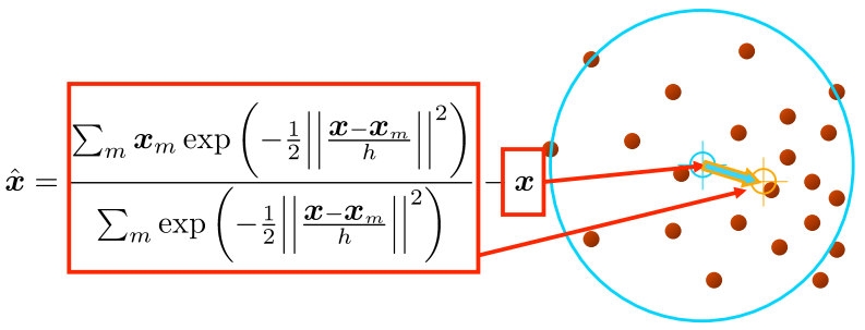
Now, for each point in our data, we can calculate a weighted mean of the points in its neighborhood, defined by the kernel. This weighted mean tells us how much we should "shift" our current point to move towards areas of higher density. Mathematically, the mean shift vector $m(x)$ is given by:

This gives us the new location after one shift. The algorithm iteratively repeats this shifting process for each data point until it converges to a mode.

The Mean Shift Vector

The mean shift vector $m(x) - x$ is calculated as the difference between the original point $x$ and the new estimate of the mean $m(x)$. The idea is that the data points are "pulled" toward the mode by this vector, much like a gravitational field.

In each iteration, we update the current point $x$ with the new mean estimate $m(x)$:

This continues until the shifts become negligible, and the points converge to their respective cluster centers.

Kernel Choices

The performance and outcome of mean shift are highly dependent on the choice of the kernel function. The most common kernel used is the Gaussian kernel, given by:

where $\sigma$ controls the width or bandwidth of the kernel.

Another common kernel is the flat kernel (a.k.a. uniform kernel), which simply assigns equal weights to all points within a fixed distance:

The choice of kernel and bandwidth $h$ (or $\sigma$ for the Gaussian kernel) is crucial and can greatly affect the clustering outcome.

Mathematical Formulation

Let's now take a deeper look into the equations involved. Consider a finite set of data points $S = \{x_1, x_2, \dots, x_n\}$ in an $n$-dimensional Euclidean space $\mathbb{R}^n$.

1. Kernel Density Estimation (KDE):

We estimate the density around each point using a kernel $K$, which is a non-negative function that integrates to 1:

Here, $h$ is the bandwidth of the kernel, which determines how far-reaching the influence of each data point is.

2. Mean Shift Vector:

We compute the mean shift vector $m(x)$ as the weighted mean of the data points within the neighborhood defined by the kernel:

This moves each point towards regions of higher density. The iterative update rule becomes:

This process repeats until convergence.

3. Convergence:

Mean shift will keep moving points until no significant shift occurs, i.e., when $m(x) - x$ is below a certain threshold. In practice, this means that the points settle into clusters, with each cluster center representing a mode of the density function.

Python Code Example

Now, let's walk through a Python implementation using scikit-learn's built-in mean shift functionality, followed by a custom implementation for a deeper understanding.

The mean shift algorithm seeks modes of the given set of points

1. Choose kernel and bandwidth
2. For each point: a) Center a window on that point b) Compute the mean of the data in the search window c) Center the search window at the new mean location d) Repeat (b,c) until convergence
3. Assign points that lead to nearby modes to the same cluster

Scikit-learn Implementation

import numpy as np
import matplotlib.pyplot as plt
from sklearn.cluster import MeanShift

## Generating synthetic data
from sklearn.datasets import make_blobs
X, _ = make_blobs(n_samples=500, centers=3, cluster_std=0.60, random_state=0)

## Applying MeanShift
ms = MeanShift(bandwidth=2)
ms.fit(X)
labels = ms.labels_
cluster_centers = ms.cluster_centers_

## Plotting the results
plt.scatter(X[:, 0], X[:, 1], c=labels, cmap='viridis')
plt.scatter(cluster_centers[:, 0], cluster_centers[:, 1], s=300, c='red')
plt.show()

Custom Implementation

Below is a simplified custom mean shift implementation to show the underlying process:

import numpy as np

def gaussian_kernel(distance, bandwidth):
    return np.exp(-0.5 * (distance / bandwidth) ** 2)

def mean_shift(X, bandwidth, max_iter=300):
    points = np.copy(X)
    for it in range(max_iter):
        for i, point in enumerate(points):
            distances = np.linalg.norm(X - point, axis=1)
            weights = gaussian_kernel(distances, bandwidth)
            weighted_sum = np.sum(X.T * weights, axis=1)
            points[i] = weighted_sum / np.sum(weights)
    
    return points

## Generating synthetic data
from sklearn.datasets import make_blobs
X, _ = make_blobs(n_samples=300, centers=4, cluster_std=0.70, random_state=0)

## Applying custom mean shift
shifted_points = mean_shift(X, bandwidth=2)

## Plotting the results
import matplotlib.pyplot as plt
plt.scatter(X[:, 0], X[:, 1], label='Original Points')
plt.scatter(shifted_points[:, 0], shifted_points[:, 1], label='Shifted Points', c='red')
plt.legend()
plt.show()

Visualization of Mean Shift in Action

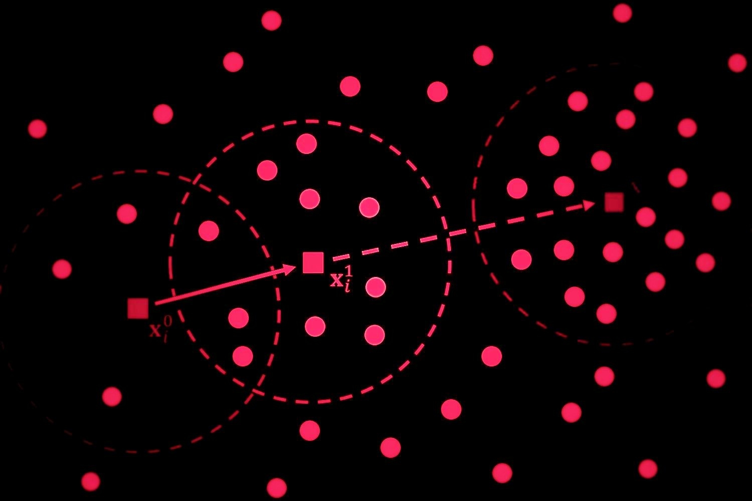
Imagine you have a circular kernel (or window) sweeping over your data points. At each iteration, the center of the kernel is moved to the mean of the points within its radius, shifting it toward denser regions of data until it settles at a peak (mode).

Here's an illustrative example of how the process works:

1. Initially, the kernel is placed at a random point in the feature space.
2. The kernel shifts iteratively towards regions with higher data density (indicated by arrows).
3. Eventually, it converges to the mode, where no further significant shift occurs.

Applications of Mean Shift

1. Clustering

Mean shift is widely used in clustering tasks. Unlike k-means, which requires the number of clusters to be predefined, mean shift adapts dynamically, making it a great fit for applications where the number of clusters is not known in advance.

2. Image Segmentation and Smoothing

In image processing, mean shift is used for tasks like image segmentation, where it helps group pixels into distinct regions. It's also employed in smoothing images, particularly using the joint spatial-range domain, to remove noise while preserving edges.

3. Object Tracking

In computer vision, mean shift can be used for object tracking. By creating a probability density function of the object's appearance in consecutive frames, mean shift tracks the object by converging to the peak of the PDF.

Strengths and Weaknesses

Strengths:

• No need to predefine the number of clusters.
• Capable of handling non-linearly separable data.
• Applicable to a wide range of problems, including image processing and feature space analysis.

§ Good general-practice segmentation § Flexible in number and shape of regions § Robust to outliers

Weaknesses:

• Computationally expensive, especially for large datasets.
• Highly sensitive to the choice of bandwidth $h$.
• Convergence is not guaranteed for all kernel functions in high-dimensional spaces.

Have to choose kernel size in advance § Not well suited for high-dimensional features

Conclusion

The mean shift algorithm is a powerful tool for clustering and density estimation, especially in scenarios where you don't want to make assumptions about the number of clusters in advance. By iteratively shifting data points towards higher-density regions, it finds the modes of a probability distribution

in a non-parametric way.

Its flexibility makes it a popular choice for various applications, including computer vision and feature space analysis, but its computational complexity can be a drawback for larger datasets.

Next Steps

• Experiment with different kernel bandwidths to see how they affect the clustering.
• Implement mean shift from scratch in Python and apply it to a real-world dataset.
• Dive deeper into applications like image segmentation or object tracking to see the algorithm's versatility.

Happy clustering!

Mean Shift Algorithm: A Gentle Dive Into Mode-Seeking

Alright, so you've probably heard of clustering algorithms like K-Means and DBSCAN, but today, we're talking about Mean Shift — one of the coolest unsupervised learning algorithms that often doesn't get enough attention. It's like K-Means but with fewer constraints, and it's got this great "mode-seeking" vibe to it.

What is Mean Shift?

Mean Shift is all about finding modes (aka peaks) in a data distribution. If you imagine your data points as little hills on a landscape, Mean Shift helps us find the tops of those hills. It doesn't need you to specify the number of clusters in advance, which is pretty awesome.

The algorithm works by shifting each data point towards the densest part of the dataset — basically moving towards the center of mass of nearby points iteratively. Over time, points converge toward their nearest mode. This is how clusters naturally form.

Let's break it down.

Step-by-step Breakdown

1. Initializing the Centroids (not explicitly)

Unlike K-Means, where you initialize specific centroids, here you start by considering every data point as a potential centroid. No need to specify k or anything — nice, right?

2. Kernel Density Estimation

Mean Shift uses something called a kernel density estimation (KDE) to estimate the density of points around each data point. You can think of it as a smooth curve fitted over your data, where "peaks" correspond to regions of high density.

The KDE formula typically involves a kernel function (often Gaussian), which gives higher weights to points that are closer to the data point of interest.

Where:

• $f(x)$ is the estimated density at point $x$
• $x_i$ are the data points
• $h$ is the bandwidth (think of it as a smoothing parameter)
• $K$ is the kernel function (often a Gaussian function)

So, for each point $x_i$, we're basically summing up the kernel values of all other points weighted by their distance.

3. Mean Shift Vector

Now comes the fun part. For each point, we compute the mean shift vector, which is essentially the difference between the current position and the weighted mean of nearby points (within a certain radius defined by the bandwidth).

Mathematically, the mean shift vector for a point $x_i$ is given by:

Where $N(x_i)$ is the neighborhood around $x_i$ defined by the bandwidth. This vector basically tells us where the data point needs to shift to move closer to a high-density region.

4. Shift the Points

Now, simply update the data point's location using the mean shift vector:

This process is repeated for all points until convergence, i.e., when the shifts are really small, or points stay in the same place.

5. Convergence and Clustering

After enough iterations, each point will converge to a mode (i.e., a high-density region). Once this happens, you can assign points that converge to the same mode to the same cluster. This is super intuitive because points in the same high-density region belong together.

Bandwidth: The Secret Sauce

Now, let's talk about the bandwidth $h$. This is one of the most important hyperparameters in Mean Shift, and it controls the size of the neighborhood around each point.

• Small bandwidth: You get a lot of clusters (probably too many), because you're focusing on really local regions.
• Large bandwidth: You might end up merging a bunch of clusters together, even though they're distinct.

So, bandwidth is a bit like Goldilocks' porridge — find the one that's "just right" for your data.

Visualization Time!

If you were to visualize Mean Shift in action, imagine dropping a bunch of marbles on a bumpy surface. Each marble represents a data point. As the algorithm progresses, the marbles roll upwards, following the slope, until they reach the peaks — those modes of high density. Once there, they stop. Marbles at the same peak belong to the same cluster.

Mathematics Behind Mean Shift

Okay, let's get a little math-heavy (because, why not?). If you're into optimization, you'll love this: Mean Shift can be interpreted as a gradient ascent on a density function. Yup, it's a fancy way of climbing a hill.

Consider the density function $p(x)$. We want to find the modes of this function by following the gradient. The gradient of a kernel density estimator (with a radially symmetric kernel) is proportional to the mean shift vector:

This is why the points move in the direction of the highest density. We're climbing the steepest part of the KDE "hill."

Advantages of Mean Shift

1. No need to predefine the number of clusters: Unlike K-Means, you don't need to know the number of clusters in advance. The algorithm just finds them for you.
2. Versatile: It works well in scenarios where clusters don't necessarily have a spherical shape. (K-Means assumes clusters are roughly spherical, which isn't always true.)
3. Mode-seeking: It directly finds the modes, which is sometimes more intuitive for clustering tasks.

Disadvantages of Mean Shift

1. Computationally expensive: Mean Shift involves repeatedly shifting all points, which can be slow for large datasets.
2. Bandwidth selection is tricky: Finding the right bandwidth can be a challenge, and there's no universal solution for choosing it.
3. Sensitive to density estimation: The quality of your clusters depends heavily on how well your kernel density estimation represents the data.

When Should You Use Mean Shift?

Mean Shift is especially useful when you don't know the number of clusters upfront, and you believe the clusters could be arbitrarily shaped. It works great for image segmentation, object tracking, and scenarios where clusters may be unevenly distributed or even noisy.

However, for very large datasets, you might want to look into approximate versions of Mean Shift (such as using KD-trees for faster neighbor searches) or even alternative methods if scalability is a concern.

Conclusion

So there you have it — Mean Shift in all its mode-seeking glory! It's a powerful clustering algorithm that can uncover complex structures in your data without making too many assumptions. While it's not the fastest kid on the block, it's got a unique charm and can handle some pretty tricky clustering scenarios. Now go forth and experiment with Mean Shift!